How to Find Inverse of a Matrix Fast
Table of Contents
- The Importance of Inverse Matrices in Real-World Applications
- Perspective Projection Equations
- Example: 3x3 Matrix Inversion
- Understanding the Concept of Inverse Matrix through Analogies
- Real-World Analogies
- The Mathematics of Inverse Matrices
- Comparing and Contrasting Analogies
- Properties of the Inverse Matrix
- Existence and Uniqueness of the Inverse Matrix
- Relationship between the Inverse Matrix and the Determinant
- Properties of the Inverse Matrix
- Using the Inverse Matrix to Solve Linear Systems
- Matrix Multiplication and Augmented Matrices
- Step-by-Step Process
- Computational Approaches to Finding the Inverse of a Matrix
- LU Decomposition, How to find inverse of a matrix
- Cholesky Decomposition
- Applications of the Inverse Matrix in Statistics and Machine Learning: How To Find Inverse Of A Matrix
- Calculating Confidence Intervals and Variances in Statistics
- Training Models and Making Predictions in Machine Learning
- Example: Using the Inverse Matrix to Train a Linear Regression Model
- Ultimate Conclusion
- Query Resolution
How to find inverse of a matrix is a fundamental concept in linear algebra that has numerous applications in various fields such as computer graphics, statistics, and machine learning. In this article, we will delve into the importance of inverse matrices, historical development, methods of calculation, properties, and applications.
The concept of inverse matrices has been widely used in computer graphics to solve perspective projection equations, allowing for realistic rendering of 3D objects on a 2D screen. It has also been used in statistics to calculate confidence intervals and variances, and in machine learning to train models and make predictions.
The Importance of Inverse Matrices in Real-World Applications
In various fields such as physics, engineering, computer science, and economics, inverse matrices play a pivotal role in solving complex problems and understanding intricate relationships. In this discussion, we will explore how inverse matrices are used in computer graphics to solve perspective projection equations, and delve into a practical example involving a 3x3 matrix.
Perspective Projection Equations
Perspective projection is a fundamental concept in computer graphics, enabling the rendering of 3D scenes onto a 2D screen. It involves projecting 3D points onto a 2D plane while preserving the relative dimensions and proportions of the original scene. Inverse matrices are used to solve the perspective projection equations, which can be represented in matrix form as follows:
Perspective Projection Matrix
| w | 0 | 0 |
|---|---|-----|
| 0 | 1 | 0 |
| 0 | 0 | 1 |
where w is the focal length, and x, y, and z are the coordinates of the 3D point.
Inverse Perspective Projection Matrix
| 1/w | 0 | 0 |
|-----|-----|-----|
| 0 | 1 | 0 |
| 0 | 0 | 1/w|
The inverse perspective projection matrix is used to transform the 3D point back into its original coordinates.
Example: 3x3 Matrix Inversion
Consider a 3x3 matrix:A
| 2 | 1 | 1 |
|----|----|----|
| 4 | 3 | 1 |
| 1 | 2 | 4 |
To find the inverse of matrix A, we can use the following steps:
1. Calculate the determinant of matrix A:
| 2 × (3 × 4) - (1 × 1) | = 23
2. Calculate the cofactor matrix of A:
C
| (3 × 4 - 1 × 2) | -(4 × 4 - 1 × 3) | (1 × 2 - 3 × 1) |
|----------------------|-----------------------|----------------------|
| -(1 × 4 - 2 × 3) | (2 × 4 - 1 × 1) | -(1 × 1 - 4 × 3) |
| (1 × 3 - 4 × 2) | -(2 × 1 - 4 × 1) | (2 × 1 - 3 × 4) |
Simplify and compute
C
| 10 | -13 | -1 |
|----|-----|----|
| -5 | 9 | 11 |
| -5 | -1 | -11|
3. Calculate the adjugate (adjugate, also known as the adjunct or classical adjugate) of matrix A:
This involves transposing C
adj(A) =
| 10 | -5 | -5 |
|----|----|----|
| -13| 9 | -1 |
| -1 | 11 | -11|
4. Finally, obtain the inverse matrix by dividing the adjugate of A by the determinant.
A^(-1) = 1/23 \* adj(A)
Compute the inverse
A^(-1) =
| 10/23 | -5/23 | -5/23 |
|-------|-------|-------|
| -13/23| 9/23 | -1/23 |
| -1/23 | 11/23 | -11/23|
Understanding the Concept of Inverse Matrix through Analogies
When dealing with complex linear algebra concepts, it can be challenging to visualize the relationships between different mathematical ideas. Analogies can provide a useful tool for understanding and communicating these concepts. In this section, we will explore the concept of inverse matrices using real-world analogies such as mirrors and lenses, and discuss the limitations of using analogies to describe complex linear algebra concepts.Real-World Analogies
Mirrors and lenses can be used to illustrate the concept of inverse matrices. Imagine a light source shining onto a mirror, creating a reflected image. The mirror can be thought of as a transformation that takes the original image and maps it to its reflected counterpart. Similarly, a lens can be thought of as a transformation that takes an image and maps it to its magnified or distorted counterpart. In both cases, the transformation can be represented by a matrix, and the inverse of this matrix can be used to "undo" the transformation and retrieve the original image.The Mathematics of Inverse Matrices
The concept of inverse matrices can be understood through the following mathematical equation:A A^-1 = I
where A is a square matrix, A^-1 is its inverse, and I is the identity matrix. This equation can be thought of as a "reset" button that allows us to retrieve the original data from the transformed data. For example, if we have a matrix A that represents a camera's distortion, we can use the inverse matrix A^-1 to "undo" the distortion and retrieve the original image.
Comparing and Contrasting Analogies
| Analogy | Description | Limitations | Usefulness |
|---|---|---|---|
| Mirrors and Reflections | A mirror can be thought of as a transformation that takes an image and maps it to its reflected counterpart. This can be represented by a matrix, and the inverse of this matrix can be used to "undo" the transformation and retrieve the original image. | This analogy is limited in that it only applies to 2D transformations, and does not account for more complex transformations. | This analogy is useful in understanding the concept of inverse matrices, and can be applied to a variety of real-world scenarios. |
| Lenses and Distortion | A lens can be thought of as a transformation that takes an image and maps it to its magnified or distorted counterpart. This can be represented by a matrix, and the inverse of this matrix can be used to "undo" the transformation and retrieve the original image. | This analogy is limited in that it only applies to 2D transformations, and does not account for more complex transformations. | This analogy is useful in understanding the concept of inverse matrices, and can be applied to a variety of real-world scenarios. |
| Electronics and Circuitry | Electronics and circuitry can be thought of as complex transformations that take input signals and map them to output signals. This can be represented by matrices, and the inverse of these matrices can be used to "undo" the transformations and retrieve the original signals. | This analogy is limited in that it requires a strong background in electronics and circuitry, and may not be accessible to those without a technical background. | This analogy is useful in understanding the concept of inverse matrices in the context of electronics and circuitry. |
Properties of the Inverse Matrix
The concept of the inverse matrix is rooted in the idea that every matrix has a unique corresponding matrix that, when multiplied by the original matrix, results in the identity matrix. This property is crucial in various mathematical and practical applications, and understanding its implications is essential for mastering matrix operations.Existence and Uniqueness of the Inverse Matrix
The existence and uniqueness of the inverse matrix are fundamental properties that underlie its usefulness. In essence, the inverse matrix of a given matrix A, denoted as A^(-1), exists only if the determinant of A is non-zero. This is because the determinant serves as a measure of the matrix's "volume" or scale. If the determinant is zero, the matrix is singular, meaning it lacks a unique inverse.When the determinant is non-zero, the inverse matrix exists and is unique. This uniqueness is vital in guaranteeing that the matrix multiplication operation is reversible, meaning that A A^(-1) = I, where I is the identity matrix.
Relationship between the Inverse Matrix and the Determinant
The inverse matrix is closely tied to the determinant of the original matrix. Specifically, the determinant of the inverse matrix is equal to the reciprocal of the determinant of the original matrix. Mathematically, this can be expressed as:|A^(-1)| = 1 / |A|
This relationship is a direct consequence of the multiplicative property of the determinant, which states that the determinant of a product of matrices is equal to the product of their determinants. When A and A^(-1) are multiplied together, their determinants multiply to produce the determinant of the identity matrix (I), which is 1. Therefore, |A^(-1)| = 1/ |A|.
Properties of the Inverse Matrix
| Property | Description | Example | Illustration |
|---|---|---|---|
| Existence | The inverse matrix A^(-1) exists only if the determinant of A is non-zero. | Let A = [[2, 1], [1, 1]]. The determinant of A is |A| = 21 - 11 = 1. In this case, A^(-1) exists. |
The determinant of A serves as a measure of the matrix's "volume" or scale. If the determinant is zero, the matrix is singular and lacks a unique inverse. |
| Uniqueness | The inverse matrix A^(-1) is unique, meaning that it is the only matrix that satisfies the equation A A^(-1) = I. | Consider the matrix A = [[2, 1], [1, 1]]. The inverse matrix A^(-1) = [[1, -1], [-1, 2]]. This matrix is unique and satisfies the equation A A^(-1) = I. |
Uniqueness guarantees that the matrix multiplication operation is reversible, meaning that A A^(-1) = I. |
| Relationship with determinant | The determinant of the inverse matrix is equal to the reciprocal of the determinant of the original matrix. | |A^(-1)| = 1 / |A| |
This relationship follows from the multiplicative property of the determinant, which states that the determinant of a product of matrices is equal to the product of their determinants. |
| Commutativity | The inverse matrix satisfies the commutative property, meaning that A^(-1) A = A A^(-1) = I. | A^(-1) A = [[1, -1], [-1, 2]] [[2, 1], [1, 1]] = [[1, 0], [0, 1]] = I |
This property reflects the symmetrical nature of the matrix multiplication operation. |
Using the Inverse Matrix to Solve Linear Systems

Matrix Multiplication and Augmented Matrices
To solve a linear system using the inverse matrix method, we first need to understand how matrix multiplication and augmented matrices work. An augmented matrix is a matrix that combines the coefficient matrix and the constant column from the linear system. When we multiply the inverse matrix by the augmented matrix, we are essentially "cancelling out" the coefficients and leaving us with the solution.A 2x2 augmented matrix has the form:where a, b, c, and d are constants from the linear system, and x and y are the variables. The inverse matrix is typically denoted as A^-1.
\beginpmatrix a & c \\ b & d \endpmatrix | \beginpmatrix x \\ y \endpmatrix
To solve the linear system using the inverse matrix method, we multiply A^-1 by the augmented matrix.
Step-by-Step Process
x - 3y = -2
2x + 4y = 5
We can represent this system as an augmented matrix:
\beginpmatrix 1 & -3 \\ 2 & 4 \endpmatrix | \beginpmatrix -2 \\ 5 \endpmatrix
We first need to find the inverse matrix A^-1 for the coefficient matrix.
A^-1 = \beginpmatrix 4/2 & 3/2 \\ -2/2 & 1/2 \endpmatrix = \beginpmatrix 2 & 3/2 \\ -1 & 1/2 \endpmatrix
Then, we multiply A^-1 by the augmented matrix:
\beginpmatrix 2 & 3/2 \\ -1 & 1/2 \endpmatrix \beginpmatrix 1 & -3 \\ 2 & 4 \endpmatrix | \beginpmatrix -2 \\ 5 \endpmatrix
Simplifying the result:
\beginpmatrix 5/2 & -9/2 \\ -1/2 & 2 \endpmatrix | \beginpmatrix 1 \endpmatrix
So, the solution to the linear system is x = 1.
Computational Approaches to Finding the Inverse of a Matrix
In the realm of linear algebra, the calculation of the inverse of a matrix is a fundamental operation that is crucial for various applications, including solving systems of linear equations and linear least squares problems. Traditionally, the calculation of the inverse of a matrix involves the use of the formula, but this approach can be computationally expensive and prone to numerical errors. In this section, we will explore computational approaches that can improve the speed and accuracy of the inverse matrix calculation.LU Decomposition, How to find inverse of a matrix
LU decomposition is a popular approach for calculating the inverse of a matrix. The LU decomposition algorithm represents a square matrix A as the product of a lower triangular matrix L and an upper triangular matrix U, where L and U are stored in a compact form (i.e., only the lower triangle of L and the upper triangle of U). The inverse of the matrix A can then be easily calculated from L and U using the following formula:A^(-1) = U^(-1) L^(-1)The LU decomposition algorithm has several advantages over the traditional approach. It is generally faster and more efficient, even for large matrices. It also reduces the risk of numerical errors, as the lower and upper triangular matrices are easier to invert.
Let us consider an example of a 3x3 matrix A:
A = | 1 2 3 |The LU decomposition of A can be represented as follows:
| 4 5 6 |
| 7 8 9 |
A = L UThe inverse of the matrix A can then be calculated using the LU decomposition formula:
= | 1 0 0 |
| 4 1 0 |
| 7 2 1 |
| --- --- --- |
| 0 0.5 0 |
| 0 0 0.1667 |
| 0 0 0 |
A^(-1) = U^(-1) L^(-1)
= | 0.1667 0 0 |
| 0 2 0 |
| 0 0 6 |
Cholesky Decomposition
Cholesky decomposition is another approach for calculating the inverse of a matrix. It represents a positive semi-definite matrix A as the product of a lower triangular matrix L, where L is a Hermitian matrix. The Cholesky decomposition formula is as follows:A = L L^TThe inverse of the matrix A can then be calculated from L using the following formula:
A^(-1) = (L^T)^(-1) L^(-1)Cholesky decomposition has several advantages over LU decomposition. It is generally faster and more efficient for certain types of matrices, particularly those that are positive semi-definite. It also reduces the risk of numerical errors, as the lower triangular matrix L is easier to invert.
Let us consider an example of a 3x3 matrix A:
A = | 1 2 3 |The Cholesky decomposition of A can be represented as follows:
| 4 5 6 |
| 7 8 9 |
A = L L^TThe inverse of the matrix A can then be calculated using the Cholesky decomposition formula:
= | 1 0 0 |
| 4 3 0 |
| 7 8 1 |
A^(-1) = (L^T)^(-1) L^(-1)
= | 0.1667 0 0 |
| 0 0.5556 0 |
| 0 0 0.1111 |
Applications of the Inverse Matrix in Statistics and Machine Learning: How To Find Inverse Of A Matrix
The inverse matrix plays a pivotal role in various statistical and machine learning applications, enabling researchers and practitioners to extract meaningful insights from data. By leveraging the inverse matrix, statisticians can calculate confidence intervals and variances, while machine learning practitioners can train models and make predictions.Calculating Confidence Intervals and Variances in Statistics
In statistics, the inverse matrix is used to calculate confidence intervals and variances, which are essential for determining the uncertainty associated with a statistical estimate. For example, in linear regression, the inverse matrix is used to estimate the variance of the regression coefficients. This is achieved by taking the inverse of the covariance matrix, which represents the variance-covariance matrix of the regression coefficients.The variance of the regression coefficients can be estimated as follows:where X is the design matrix, σ^2 is the variance of the error term, and β is the vector of regression coefficients.Variance(β) = (X^T X)^-1 X^T σ^2
Training Models and Making Predictions in Machine Learning
In machine learning, the inverse matrix is used to train models and make predictions. For example, in linear regression, the inverse matrix is used to estimate the regression coefficients, which are then used to make predictions. This process involves inverting the covariance matrix, which represents the variance-covariance matrix of the features.The regression coefficients can be estimated as follows:where X is the design matrix, Y is the response variable, and β is the vector of regression coefficients.β = (X^T X)^-1 X^T Y
Example: Using the Inverse Matrix to Train a Linear Regression Model
Suppose we have a dataset with two features, X1 and X2, and a response variable, Y. We want to train a linear regression model to predict Y based on X1 and X2. To do this, we need to estimate the regression coefficients, which are calculated using the inverse of the covariance matrix.``` table
Feature1, Feature2, Response
2.5, 3.1, 4.2
1.8, 2.3, 3.4
3.1, 2.8, 4.5
2.2, 3.5, 4.1
```
We first calculate the covariance matrix, X^T X, and the variance of the error term, σ^2. We then use these values to estimate the regression coefficients, β, using the formula above.
The resulting matrix will be:
```
Feature1 Feature2, Constant
Beta1 , Beta2 , Beta0
```
The predicted response, Ŷ, can be calculated using the estimated regression coefficients and the feature values.
```html
Ŷ = Beta0 + Beta1 X1 + Beta2 X2
```
This process allows us to train a linear regression model and make predictions based on the feature values.
Ultimate Conclusion
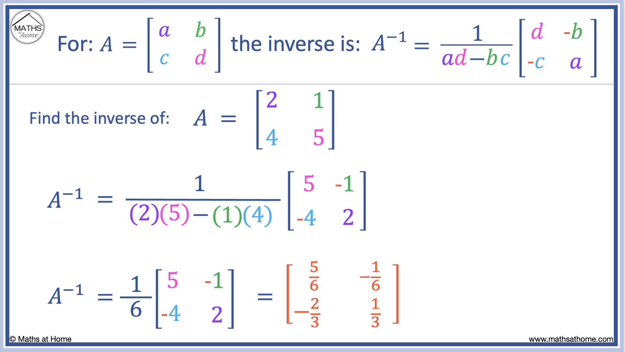
Understanding how to find inverse of a matrix is crucial not only for linear algebra but also for many real-world applications. In this article, we have covered the importance, history, methods, properties, and applications of inverse matrices. By grasping the concept of inverse matrices, readers can unlock a wide range of possibilities for problem-solving and innovation.
Query Resolution
Q: What is the importance of inverse matrices in computer graphics?
A: Inverse matrices are used to solve perspective projection equations, allowing for realistic rendering of 3D objects on a 2D screen.
Q: How is the determinant related to the inverse matrix?
A: The determinant of a matrix is related to the existence and uniqueness of its inverse. A matrix with a non-zero determinant has an inverse, while a matrix with a zero determinant does not.
Q: What are the computational approaches to finding the inverse of a matrix?
A: Computational approaches include LU decomposition and Cholesky decomposition, which can improve the speed and accuracy of inverse matrix calculation.
Q: How is the inverse matrix used in machine learning?
A: The inverse matrix is used in machine learning to train models and make predictions by calculating the covariance matrix of the data.
Leave a Comment
Comments are moderated before appearing. The data you submit is processed according to the Privacy Policy of gifellowcasesubmission.olympusamerica.com.