How to Calculate Asymptotes and Understand Their Significance
Table of Contents
- Understanding the Concept of Asymptotes in Mathematics
- Types of Asymptotes
- Vertical Asymptotes
- Horizontal Asymptotes
- Oblique Asymptotes
- Types of Asymptotes and Their Identification
- Horizontal Asymptotes
- Vertical Asymptotes
- Slant Asymptotes
- Imaginary Asymptotes, How to calculate asymptotes
- Analyzing Asymptotes with Graphing Calculators: How To Calculate Asymptotes
- Using Graphing Calculators to Visualize Asymptotes
- Limits of Graphing Calculators
- Exploring the Behavior of Functions Around Asymptotes
- Best Practices for Using Graphing Calculators
- Closing Notes
- Expert Answers
Delving into how to calculate asymptotes, this introduction immerses readers in a journey of exploring mathematical functions and discovering their secrets. Asymptotes are a crucial component of mathematical functions, determining their behavior and shape as they approach positive or negative infinity.
The concept of asymptotes plays a significant role in graphing and analyzing polynomial and rational functions, allowing mathematicians to visualize and understand the behavior of these functions more effectively. In this article, we will delve into the world of asymptotes, exploring their types, significance, and methods for calculating them.
Understanding the Concept of Asymptotes in Mathematics
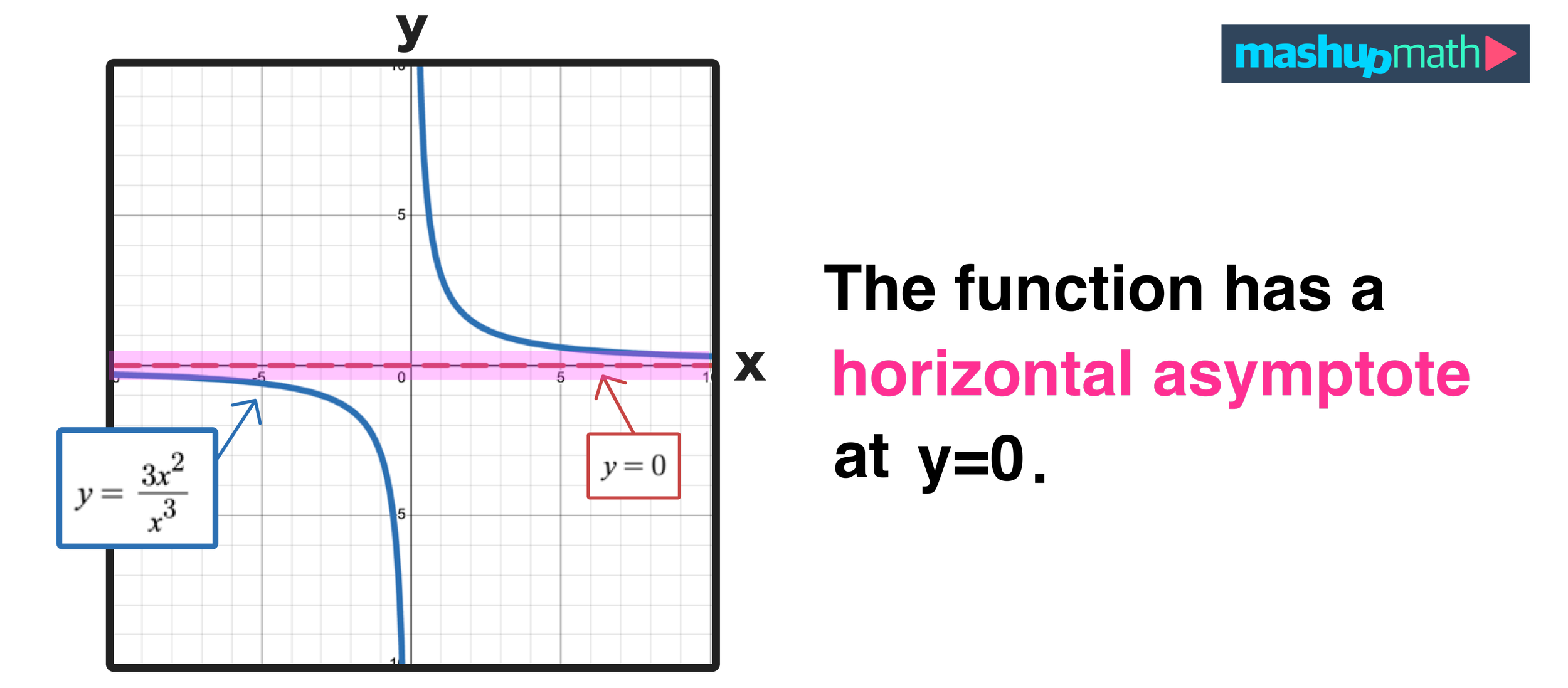
Asymptotes play a crucial role in mathematics, particularly when graphing and analyzing polynomial and rational functions. They help us understand the behavior of functions as x approaches infinity or negative infinity. In this section, we will delve into the world of asymptotes and explore their significance in mathematical functions.
Types of Asymptotes
Asymptotes can be classified into three main types: vertical, horizontal, and oblique asymptotes. Each type of asymptote provides a unique insight into the behavior of a function.
Vertical Asymptotes
Vertical asymptotes occur when a function approaches infinity or negative infinity as x approaches a specific value. This value is often denoted as c, and it represents a point where the function is undefined. The graph of a function will tend to increase or decrease infinitely as x approaches this value from either side. The general form of a rational function that exhibits a vertical asymptote is f(x) = a/x^2, where a is a constant.
- A vertical asymptote occurs when the function approaches infinity as x gets arbitrarily close to c.
- Vertical asymptotes can be found by examining the factors of the denominator in a rational function.
Horizontal Asymptotes
Horizontal asymptotes occur when a function approaches a constant value as x approaches infinity or negative infinity. This value is often denoted as y, and it represents the behavior of the function in the long run. The general form of a rational function that exhibits a horizontal asymptote is f(x) = a/x, where a is a constant.
- A horizontal asymptote determines the long-term behavior of a function.
- Horizontal asymptotes can be found by examining the degrees of the numerator and denominator of a rational function.
Oblique Asymptotes
Oblique asymptotes occur when a function approaches a linear function as x approaches infinity or negative infinity. This linear function is often denoted as y = mx + b, where m is the slope and b is the y-intercept. The general form of a rational function that exhibits an oblique asymptote is f(x) = ax + b/x, where a and b are constants.
- An oblique asymptote represents the long-term behavior of a function in a linear form.
- Oblique asymptotes can be found by performing polynomial division between the numerator and denominator of a rational function.
Asymptotes provide a powerful tool for analyzing and understanding the behavior of functions. By identifying and classifying asymptotes, we can gain insights into the long-term behavior of a function and make informed decisions about its applications.
Types of Asymptotes and Their Identification
The identification of asymptotes is a crucial step in understanding the behavior of a function, especially when it comes to determining its end behavior and graph. Asymptotes can be classified into several types, each with its own method of identification.
Horizontal Asymptotes
Horizontal asymptotes are a type of asymptote that occurs when the function approaches a constant value as the input variable approaches positive or negative infinity. To determine the horizontal asymptote of a function, we can use the following methods:
Method 1: Divide the numerator and denominator by the highest power of the variable in the denominator
When the degrees of the numerator and denominator are the same, the horizontal asymptote is given by the ratio of the leading coefficients.
y = lim x→∞ (f(x)) / x^n = a_n / b_n
When the degree of the numerator is less than the degree of the denominator, the horizontal asymptote is y = 0.When the degree of the numerator is greater than the degree of the denominator, there is no horizontal asymptote, but a slant asymptote may exist.
When the degree of the numerator is equal to the degree of the denominator, the horizontal asymptote is given by the ratio of the leading coefficients.
Method 2: Use the limit of the function as x approaches infinity or negative infinity
This method involves directly evaluating the limit of the function as x approaches infinity or negative infinity.
lim x→∞ f(x) = L
If the limit exists, then the horizontal asymptote is y = L.If the limit does not exist, then there is no horizontal asymptote.
For rational functions, we can also use the fact that the horizontal asymptote is the quotient of the leading coefficients of the numerator and denominator, provided that the degree of the numerator is less than or equal to the degree of the denominator.
y = lim x→∞ f(x) = a_n / b_n
Vertical Asymptotes
Vertical asymptotes occur when the function approaches infinity or negative infinity at a specific point. To determine the vertical asymptote of a function, we can use the following methods:Method 1: Identify the factors in the denominator
Factors in the denominator that contain a variable raised to a power will result in a vertical asymptote.
Example: f(x) = 1 / (x - 1)
In this example, the vertical asymptote is x = 1, because the denominator is equal to zero at this point.
Method 2: Use the limit of the function as x approaches the specific point
We can also use the limit of the function as x approaches the specific point to determine the existence of a vertical asymptote.
Example: f(x) = 1 / (x - 1)
In this example, the limit as x approaches 1 does not exist, indicating the presence of a vertical asymptote at x = 1.For rational functions, we can also use the fact that the vertical asymptote is the value of x that makes the denominator equal to zero, provided that the numerator is not equal to zero at this point.
y = lim x→a+ f(x) = ±∞
y = lim x→a- f(x) = ±∞
Slant Asymptotes
Slant asymptotes occur when the function approaches a linear expression as the input variable approaches infinity or negative infinity. To determine the slant asymptote of a function, we can use the following methods:Method 1: Divide the numerator and denominator by the greatest power of the variable in the denominator
When the degree of the numerator is exactly one more than the degree of the denominator, the slant asymptote is given by the quotient of the first terms in the numerator and denominator.
y = lim x→∞ f(x) = a_nx^(n-1) + a_(n-1)x^(n-2) + ... + a_0
When the degree of the numerator is exactly one more than the degree of the denominator, the slant asymptote is given by the quotient of the first terms in the numerator and denominator.
y = a_nx^(n-1) + a_(n-1)x^(n-2) + ... + a_0
Imaginary Asymptotes, How to calculate asymptotes
Imaginary asymptotes occur when the function approaches infinity or negative infinity along the imaginary axis. To determine the imaginary asymptote of a function, we can use the following methods:Method 1: Identify the factors in the denominator that contain a variable raised to a power
Factors in the denominator that contain a variable raised to a power will result in an imaginary asymptote.
Example: f(x) = 1 / (x^2 + 1)
In this example, the imaginary asymptote is y = i, because the denominator is equal to zero at this point.
Analyzing Asymptotes with Graphing Calculators: How To Calculate Asymptotes
Graphing calculators are powerful tools that can be used to visualize and explore asymptotes in functions. By using a graphing calculator, you can graph a function and observe the behavior of the function as the input values approach certain critical points, such as vertical or horizontal asymptotes. However, it's essential to note that relying solely on a graphing calculator to identify asymptotes can have limitations and potential pitfalls, as we'll discuss below. In this section, we'll explore how to use graphing calculators to explore the behavior of functions around asymptotes and discuss the importance of verifying the results using analytical methods.Using Graphing Calculators to Visualize Asymptotes
A graphing calculator can be used to visualize asymptotes by graphing a function and observing the behavior of the function as the input values approach certain critical points. For example, to visualize a vertical asymptote, enter the function and the calculator will show the asymptote as a vertical line at the critical point. Similarly, to visualize a horizontal asymptote, enter the function and observe the behavior of the function as the input values approach infinity. By graphing a function and observing the behavior of the function as the input values approach certain critical points, you can identify the asymptotes of the function.Limits of Graphing Calculators
While graphing calculators are powerful tools, they have limitations when it comes to identifying asymptotes. Firstly, the calculator may not always be able to find the exact location of the asymptote, especially if the function is complex or has multiple asymptotes. Secondly, the calculator may not always be able to distinguish between a vertical and a horizontal asymptote. Therefore, it's essential to verify the results using analytical methods, such as finding the limits of the function as the input values approach the critical points, to confirm the existence and location of the asymptotes.Exploring the Behavior of Functions Around Asymptotes
Graphing calculators can also be used to explore the behavior of functions around asymptotes by graphing the function with different window settings and observing the changes in the graph. For example, to explore the behavior of a function around a vertical asymptote, adjust the x-axis setting to narrow in on the asymptote and observe how the function behaves as the input values approach the asymptote. Similarly, to explore the behavior of a function around a horizontal asymptote, adjust the y-axis setting to zoom in on the asymptote and observe how the function behaves as the input values approach the asymptote. By graphing a function with different window settings, you can gain a deeper understanding of the behavior of the function around asymptotes.Best Practices for Using Graphing Calculators
When using a graphing calculator to analyze asymptotes, follow these best practices: Use a high-resolution graphing calculator that can accurately graph complex functions. Adjust the window settings to zoom in on the asymptotes and observe the behavior of the function. Use analytical methods, such as finding the limits of the function, to verify the existence and location of the asymptotes. Graph the function with different window settings to gain a deeper understanding of the behavior of the function around asymptotes.Closing Notes
As we conclude our exploration of how to calculate asymptotes, it is clear that these mathematical concepts have far-reaching implications in various fields, from physics to economics. By understanding asymptotes, we can better analyze and visualize mathematical functions, making informed decisions in fields reliant on mathematical modeling.
Expert Answers
Q: What are the different types of asymptotes?
A: The three main types of asymptotes are vertical, horizontal, and oblique asymptotes, each representing a distinct behavior of mathematical functions as they approach specific values of x.
Q: How do I identify vertical asymptotes in rational functions?
A: Vertical asymptotes in rational functions can be identified by finding the values that make the denominator equal to zero, and factoring the numerator to determine if removable discontinuities exist.
Q: Can asymptotes be used to model real-world scenarios?
A: Yes, asymptotes are essential in mathematical modeling, allowing us to understand and analyze complex real-world problems, and predict the behavior of systems over time.
Q: What are the limitations of graphing calculators in identifying asymptotes?
A: Graphing calculators, although useful tools, have limitations when it comes to identifying asymptotes, particularly in cases where the function has multiple asymptotes or asymptotes with complex equations.
Leave a Comment
Comments are moderated before appearing. The data you submit is processed according to the Privacy Policy of gifellowcasesubmission.olympusamerica.com.